Text Message Analyzer

Text Message Analysis with BERT Embeddings

July 2020
Reena Yuan and Nisha Prabhakar

This summer, we used our text messages as our dataset and Google's pretrained NLP model BERT to help us analyze our data in several different ways. We started off by using BERT embeddings and scikit-learn in order to classify our text messages by author. Then, we used T-SNE to visualize the embeddings and see how our conversations were affected by COVID-19. Feel free to view our code through Google COLAB.

Part 1: Text Message Classification

We wanted to see how accurate BERT embeddings, specifically for whole sentences, were by seeing how accurately they could be used to classify text messages. We did this by using the vector embeddings to train a logistic regression model.

Importing packages and libraries

We used transformers in order to use the DistilBert model, as well as several libraries including Pytorch, numpy, scikit and pandas.

!pip install transformers
import numpy as np
import pandas as pd
from sklearn.model_selection import train_test_split
from sklearn.linear_model import LogisticRegression
from sklearn.model_selection import GridSearchCV
from sklearn.model_selection import cross_val_score
import torch
import transformers as ppb
import warnings
warnings.filterwarnings('ignore')
from google.colab import files
from datetime import datetime as datetime
import io

Uploading and processing data files

Here, we uploaded Reena's text messages .csv file (which was obtained from iMessage), and reading it into a pandas dataframe. Additionally, we add a column called sender which has all values set to 0 to signify that these are Reena's texts.

NOTE: We chose to upload the data sets from our local computers because the contents (our text messages) are private.

uploaded_reena = files.upload()
df_reena = pd.read_csv(io.StringIO(uploaded_reena['test.csv'].decode('utf-8', 'ignore')), error_bad_lines=False, names=['text', 'date'])
df_reena['sender'] = [0]*len(df_reena.index)

Since the date column of df_reena is currently stored as a string, we had to convert each element in the column to a timestamp.

df_reena['date'] = df_reena['date'].apply(lambda x: pd.to_datetime(x))

Next, we uploaded a .json file containing all of Nisha's text messages. The file was downloaded from Facebook Messenger. Because of the abnormal format of the file, more cleaning had to be done.

uploaded_nisha = files.upload()

Clean is a helper method that deletes all uneccessary information from the .json file such as the reactions on a given message and what photos were sent.

def clean(dic):
dic.pop("type", None)
dic.pop("reactions", None)
dic.pop("share", None)
dic.pop("ip", None)
dic.pop("sticker", None)
dic.pop("photos", None)
dic.pop("users", None)
dic.pop("call_duration", None)
dic.pop("videos", None)
dic.pop("gifs", None)
dic.pop("files", None)
dic.pop('missed', None)
dic.pop("audio_files", None)

We read the contents of the .json file into a list called data. This method processes the dictionaries from data[1] ... the last element. In it, we delete all the extraneous data that the .json file gave us using the clean method. Also, we filtered to only include texts that Nisha sent.

def addtoDf(dic):
del dic['participants']
del dic['title']
del dic['is_still_participant']
del dic['thread_type']
del dic['thread_path']

end = []

for element in dic['messages']:
clean(element)
if(element["sender_name"] == "Nisha Prabhakar"):
element.pop("sender_name")
end.append(element)

with open("memory.json", "w") as write_file:
json.dump(end, write_file)

return pd.read_json('memory.json')

This method is called on the dictionaries in data[0]. Because the dictionary format is slightly different, we had to build a separate method to process it. It does roughly the same thing as addtoDf.

def addtoDfFirst(dic):
clean(dic)

if (dic['sender_name'] != "Nisha Prabhakar"):
return pd.DataFrame()

with open("memory.json", "w") as write_file:
json.dump(dic, write_file)

return pd.read_json('memory.json', typ='series')

This is the overarching procedure to clean the file uploaded_nisha and create one pandas dataframe that contains the data. When the data was loaded, we received a list (called data). The first element of data was a list itself, whose elements were dictionaries. On the other hand, the second element of data through the last element were dictionaries.

import json
with open('merged_file.json') as json_data:
data = json.load(json_data)
df_nisha = pd.DataFrame()
for dictionary in data[0]:
df_new = addtoDfFirst(dictionary)
df = df_nisha.append(df_new, ignore_index=True)
df_nisha = df
for i in range(1, len(data)):
df_new = addtoDf(data[i])
df = df_nisha.append(df_new, ignore_index=True)
df_nisha = df

In order to match the formats of df_reena and df_nisha, we deleted the "sender_name" column and created a new column of all 1's, which identified the texts as being written by Nisha. Additionally, we changed the other two column names to match df_reena.

del df_nisha['sender_name']
df_nisha['sender'] = [1]*len(df_nisha.index)
df_nisha.columns=['text', 'date', 'sender']
df_nisha.head()

Since there were some irregularities in Nisha's message file (some of the text messages were not of the String datatype), we iterated through each text and deleted the offending texts.

df_nisha = df_nisha[11:]
dropped = []
for index, row in df_nisha.iterrows():
if not isinstance(row['text'], str):
dropped.append(index)

df_nisha = df_nisha.drop(dropped)
df_nisha=df_nisha.sort_values(by=['date'])

For performance purposes we only used the most recent 2000 texts. We also concatenated df_nisha and df_reena and sorted the resulting df_total by date.

df_nisha_short = df_nisha[-2000:]
df_reena_short = df_reena[-2000:]
df = df_reena_short.append(df_nisha_short, ignore_index=True)
df_total = df_reena.append(df_nisha, ignore_index=True)
df_total=df_total.sort_values(by=['date'])

Extracting DistilBert embeddings

We followed this tutorial by Jay Alammar for the DistilBERT analysis.

We began by loading in the DistilBERT model and other relevant classes.

model_class, tokenizer_class, pretrained_weights = (ppb.DistilBertModel, ppb.DistilBertTokenizer, 'distilbert-base-uncased')
tokenizer = tokenizer_class.from_pretrained(pretrained_weights)
model = model_class.from_pretrained(pretrained_weights)

This method completely encodes all of the texts, from words to integer id's. After adding the special "[CLS]" and "[SEP]" tokens at the beginning and end of the texts, we tokenized the texts. The tokenizer splits up words that are not in its default dictionary into smaller parts and assigns them their associated id. Although initially we chose to maximize the length of our tokenized text array (512), this caused extracting the embeddings to use far too much RAM. We realized that only 6 of texts had more than 50 tokens, so we decided to set 50 as the maximum length of a tokenized text message.

def modified_encoder(x):
marked_text = "[CLS] " + x + " [SEP]"
tokenized_text = tokenizer.tokenize(marked_text)
indexed_tokens = tokenizer.convert_tokens_to_ids(tokenized_text[:50])
return indexed_tokens

tokenized = df['text'].apply(modified_encoder)

Here, we convert our list of tokenized texts (each text is represented as a list) into a two dimensional numpy array. This allows us to calculate the embeddings of all the texts at once.

max_len = 0
for i in tokenized.values:
if len(i) > max_len:
max_len = len(i)

padded = np.array([i + [0]*(max_len-len(i)) for i in tokenized.values])

Our array padded is a uniform array where each text is represented by an array of integers of size 50. However, we need to tell BERT to ignore the extra 0's padded onto texts whose length is less than 50, so we created an array of integers called the attention_mask.

attention_mask = np.where(padded != 0, 1, 0)

We retrieve the embeddings from the model by converting padded and attention_mask into tensors and passing them into our model.

input_ids = torch.tensor(padded)
attention_mask = torch.tensor(attention_mask)
with torch.no_grad():
last_hidden_states = model(input_ids, attention_mask=attention_mask)

Creating and training scikit model

We currently have embeddings for each word in each text. We use the first element of last_hidden_states, which is the last layer of the neural network. In order to consolidate this data into one embedding for each text, we use the embedding for the "[CLS]" token, which is the first token and often used to represent the sentence as a whole.

features = last_hidden_states[0][:,0,:].numpy()

Here we split our data into training and testing data

labels = df['sender']
train_features, test_features, train_labels, test_labels = train_test_split(features, labels)

Obtaining the logistic regression classifier and fitting it with our data was quite simple.

lr_clf = LogisticRegression()
lr_clf.fit(train_features, train_labels)

We used test_features and test_labels to see how well our model scored against the testing data. It does fairly well, with an accuracy of about 81.4%.

lr_clf.score(test_features, test_labels)

Testing our model with inputs

The prepare method converts a text string to its embeddings. This is necessary to prepare the texts to feed into our model, which is based on vectors, not strings.

def prepare(x):
tokenized = tokenizer.encode(x, add_special_tokens=True)
input_ids = torch.tensor([tokenized])
with torch.no_grad():
last_hidden_states = model(input_ids)
return last_hidden_states[0][0][0].unsqueeze(0).numpy()

The guess method calls on our model to predict who wrote the given text, and then interprets the integer returned back to a string with the person's name.

def guess():
x = input("Enter a text!")
sender = lr_clf.predict(prepare(x))[0]
if sender == 1:
return 'nisha'
else:
return 'reena'

guess()

Part 2: Visualizing BERT Embeddings

Here, we used T-SNE in order to reduce the length of our embeddings from length 768 to 2. This way we were able to visualize our sentence embeddings by plotting them on a 2-D graph.

Importing packages and libraries

We used the ski-kit machine learning library for T-SNE and matplotlib to graph our points.

from sklearn.manifold import TSNE
import matplotlib.pyplot as plt
from matplotlib.pyplot import figure

Splitting up our dataset

Due to the COVID-19 pandemic, our daily lives were significantly impacted, especially when our second semester went remote. Assuming our text messages would reflect this change, we wanted to see how our texts would look before shelter-in-place, during shelter-in-place, and after summer break started. As a result, we split up our dataset accordingly into three parts. We also had to change the step size for each dataframe in order to keep our number of texts to be around 4000.

spring_semester = datetime(2020, 1, 20)
covid = datetime(2020, 3, 9)
summer_break = datetime(2020, 5, 15)
df_precovid = df_total[(df_total['date'] > spring_semester) & (df_total['date'] < covid)].iloc[::2, :]
df_postcovid = df_total[(df_total['date'] > covid) & (df_total['date'] < summer_break)].iloc[::7, :]
df_summer = df_total[df_total['date'] > summer_break].iloc[::2, :]

Embedding and graphing

We got our sentence embeddings the same way as we did for text classification above. The graph function then uses the embeddings and authors returned by the embed function to plot the texts. The color of each point on the graph is determined by the author.

def graph(points, senders, title):
two_points = TSNE(n_components=2).fit_transform(points)
figure(figsize=(6,6))
for i, sender in enumerate(senders):
if sender == 1:
plt.scatter(two_points[i][0], two_points[i][1], marker='.', c='b')
else:
plt.scatter(two_points[i][0], two_points[i][1], marker='.', c='r')
plt.axis([-120, 120, -120, 120])
plt.title(title)
plt.show

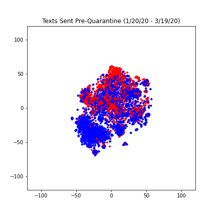
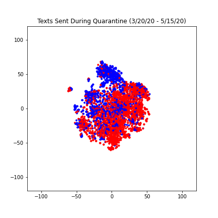
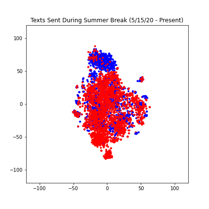
We found our results to be really interesting, especially because of the differences between the three plots. The points on the first and second graph have a much lower spread compared to the third graph. We reasoned that this is because the subject of our text messages, similar to our daily activities, became less restrained after school ended. The spread of the first and second graph are fairly similar, however the second graph is slightly more compact and the red and blue texts are less differentiable. We think this likely reflects the way Covid-19 made our daily lives even more similar than they were at Berkeley (same major, classes, dorms), the most significant similarity being quarantine.